Lecture notes for Macro I, page 1
©John Hassler, revised February 5, 1997.
Growth
The Samuelson-Diamond-Blanchard OLG model
Households
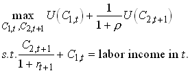
Live for two periods and solve

1
Firms
Hire labor and capital on competitive market and combine them in a CRS production function to produce the only good. This is sold on a competitive market to the households.
Firms solve
![]()
2
where At is a productivity index that grows geometrically at rate g. We can think of AL as the number of effective units of labor. Also L grows at a geometric rate n. So

3
The competitive market imply that factors are paid their marginal products. r = FK and w=FAL.
Since F is H(1) we have

4
So f is production per effective labor unit and k is capital per effective labor unit. Note that
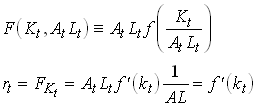
5
Since we CRS and competitive markets firms make zero profits. We can write this as

6
Note that we now see that both wages and interest rates are determined by the current capital to effective labor ratio. We thus write

7
Capital market
The labor income of a young generation in t equals wt At Lt . Part of this is consumed (c1,t) and the rest is saved. Let st denote the share of labor income that is saved. This will, in general depend on labor income and the interest rate. The savings in period t is next periods capital stock
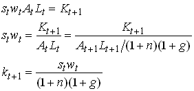
Now assume that st only depends on rt+1. (Which class of utility functions produce this result? What are the effects of higher r?) Then we can write the last line of as

This (implicitly) defines a difference equation for k, i.e., a relation between kt and kt+1 that has to be satisfied in this model. Note that if we made the Solow assumption of a constant savings rate, the difference equation takes an explicit form. Since in this case the RHS contains no kt+1. Fortunately there is a utility function for which the income and substitution effects of higher interest rates cancel so that the household will choose a constant savings rate regardless of the interest rate.
Functional specification
Let us look at a particularly simple
specification. Assume U is the log function and that that
production is (Wicksell-) Cobb-Douglas, ![]() .
.
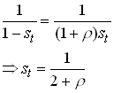
Now we can write the consumption decision of the consumer as follows.

10
with foc
11
Now we only need to specify the wage function
to have an explicit version of . We see immediately that ![]() . So becomes
. So becomes
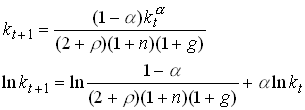
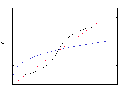
Can you solve this difference equation and is it stable? Here is an example of a plot of .
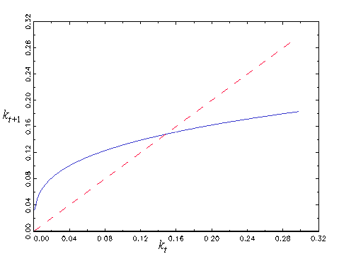
The steady state of is its fixed point

13
The interest rate in steady state is

Dynamic Inefficiency
In each time period the amount of resources is Kt + F(Kt ,AtLt). This has to be split into aggregate consumption and next periods capital stock. We can than write
![]()
15
where Ct is total consumption of young and old in period t. Now divide by At Lt

16
ct is aggregate consumption per unit of current effective unit of labor.
Now consider an economy in a steady state. We then have

17
Let us find the value of the steady state capital stock that maximizes aggregate consumption per effective unit of labor. The FOC for this problem is
![]()
This is a variant of the Ramsey Golden Rule. A steady state capital stock above kgr is not Pareto efficient. If we are above kgr we could increase aggregate consumption in all periods now and in the future by reducing forcing the steady state capital stock to be lower.
Now compare and

19
So it is possible that the economy is not on the Pareto frontier and thus dynamically inefficient. What goes wrong here and why does not the first welfare theorem hold? One way of understanding this is to realize that the only way a young generation can reduce the capital stock is by saving less but then consumption would have to be lower for them in the second period. If, however, there was a mechanism that specified that young people saved less but in return got some transfers from the young next period, everybody could be made better off. What does this remind you off?
More general savings functions
In a more general case, the difference equation given by can be less nice. It can have no or multiple steady states. With multiple steady states, some will be non-stable. Multiple steady states could occur if, for example, the savings rate increase as interest rate falls (the income effect dominates).
