
Fiscal Policy
In the neo-classical model we can think of (at least) four ways the fiscal policy affects the growth path of the economy
Government spending directly affecting production and utility functions.

58
By changing government consumption utility (production) and marginal utility (products) changes. This would cause relative prices to change. A simplification is achieved if we let government services enter additively
![]()
59
in this case g will not change the marginal utilities of goods and leisure.
Change the budget set of agents
Non-lump sum taxes which drive a wedge between MRS and MRT
Redistribute resources
The intertemporal budget set – Ricardian Equivalence
Assume the government goods do not interact with other goods in utility or production and disregard exogenous growth in population or technology. We now want to show that the path of financing of government purchases is irrelevant for the consumers. I.e., the time profile of budget deficits and taxes is irrelevant. Only the present value of government spending and the initial debt level is important.
The government budget constraint gives
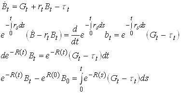
60
Now require that the present value of the debt converges
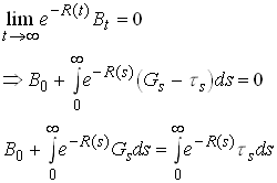
61
So the present value of all future taxes equals the present value of future government spendings plus current debt stock.
Now look at the consumers. Recall that the slope of the consumption path was given from the Euler equation.

62
As long as the tax does not affect this the slope of consumption is unaffected by the way of financing. Now look at the budget constraint. The instantaneous budget constraint is
![]()
63
Integrate
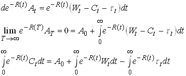
Now we can substitute into the last line of

65
so we see that what is important for the households is only the present value of government spending plus initial debt.
Some critical assumptions for the Ricardian Equivalence result
Perfect capital markets (so the individual can save or borrow to offset any changes in the time path of taxes and deficits. Same interest for government and individuals.
Taxes are lump sum.
Infinite horizons, not necessarily infinite lives.
Ricardian Equivalence with Finite lives and altruism
Consider the simplest example of this. Each generation lives for one period, cares about their kids.

66
Now we can substitute from future generations problems
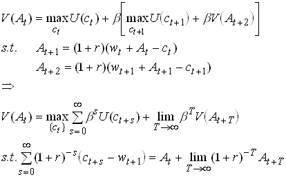
67
As you see, this is mathematically equivalent to dynamic optimization problem with infinite horizons. So the solution to this problem must be unaffected by the financing path of the governments consumption. Note that we require perfect capital markets. In this context it in particular requires that At may be negative or that households choose positive values (bequests) voluntarily.
Borrowing versus Taxing in the standard OLG model
Now let us look at whether Ricardian Equivalence holds in a standard OLG model without altruism. To focus on the path of financing rather than the spending side we consider a government which wants to finance a constant spending level of 0 for convenience. Consider a government that issues debt equal to Bt , gives the proceeds to the currently young, rolls over the debt for ever and the tax the young in all future periods to pay the interest rate minus the growth rate of the economy. This means that bt will be held constant at a level bFor simplicity let us use the log utility, Cobb-Douglas production specification.
The saving decision of the currently young given in is unaffected but the transfer has to be added to the wage

68
From this we see that current consumption increases when the policy is started up. Total savings also increase and become

69
Note that part of the savings is in form of government bonds. But it is only real savings that translate into next periods capital stock. To put it differently next periods capital stock is equal to private savings plus government savings, the latter being equal to minus Bt
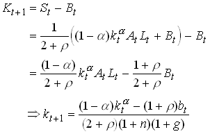
Alternatively we could derive from noting that next periods capital stock equals production plus the capital stock minus consumption.
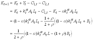 .
.
71
From we see that it is clear that the deficit financed transfer causes next periods capital stock to decrease. This means that the interest rate goes up. This in turn means that the old in the next period can consume more for each dollar saved when young. Since total savings (the sum of real and financial savings) increased, the old in t+1 will consume more. The generation born in time t when the debt was issued will this clearly benefit and we do not have Ricardian Equivalence.
From next period the government takes away an amount equal to the debt plus interest rate from the young and gives them the rolled over debt. Let Ht+1 denote total wealth of a generation born at t+1. We then have

72
We see that wealth decrease (increase) in b if the economy is dynamically efficient (inefficient). This is for given kt+1 Since the introduction of a government debt necessarily implies a lower capital stock this has negative effects on the wealth and utility of the young in t+1. For sufficiently large dynamic inefficiencies it is possible that that the first effect dominates for small debt levels.
Now consider the consumption of the young;

73
and consumption of the old is

74
Now consider the capital accumulation equation. This equals total resources available minus consumption
![]()
75
Normalizing and simplifying we get
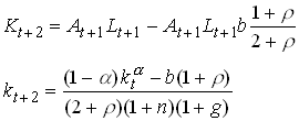
76
This follows from the fact that next periods capital stock is equal to the share of production that goes to the young minus their consumption. We see that this difference equation implies that next periods k is lower the larger is b. This implies that the new steady state capital stock is necessarily smaller when a debt roll-over is introduced.
Distortive Taxation
A positive analysis of capital taxation
Now consider the case when taxes are distortive. In this case we cannot be sure that the path of financing of a given path of spendings is irrelevant. First consider a positive analysis of capital taxation in a standard Ramsey model. The households solves
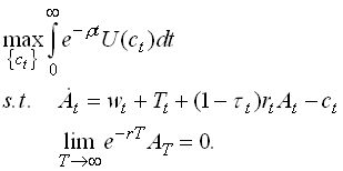
77
Competitive firms set wages and pre-tax interest rates equal to their respective marginal products. The Hamiltonian for the consumer is

78
Doing the standard trick of taking time derivatives of the optimality condition and substitute we find
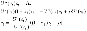
79
The phase diagram is
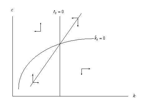
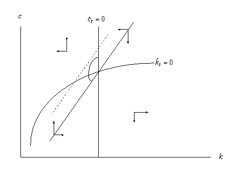
Now consider a temporary tax increase that finance a temporary increase in transfers. We assume the tax increase occurs at a time when the economy is in a steady state. In the phase diagram the tax increase implies a leftward shift in the constant consumption curve. At the time of the tax decrease we have to be at the old saddle path again. The only way this can be acheievde is indicated below. Consumption jumps, and this leads to a decrease in the capital stock. consumption then falls and at the time of the shift back it is below the constant capital curve so consumption and capital grows and the old steady state is then approached.
A normative analysis of labor taxation
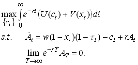
To study this consider a benevolent government that wants to finance a given but arbitrary stream of spendings {gt } with a tax on an elastic labor supply. First consider the consumer. He solves
80
where c is consumption, x is leisure and t is a potentially time varying labor tax. For simplicity we have assumed an additive utility function so that the marginal utilities are independent of other consumption.
The current value Hamiltonian is
![]()
81
with necessary condition

82
From the last condition we get that m t is constant, which implies that consumption is constant and that

So the individual we work a lot when taxes are low and vice versa.
Now consider the benevolent government. It solves
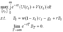
84
Since variations in the tax rate determines variations in labor supply, which is what the government is potentially worried about we can use and substitute into the governments problem.
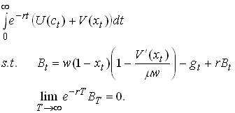
85
The current value Hamiltonian with necessary conditions for optimality becomes
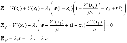
86
From the last we see that l t is constant. Using this in first order condition we get

87
If this equation has a solution it implies a constant level of xt. A case when no solution may exist is when V’’ is zero. Why is that?