Fluctuations
Consumption and Investment under Uncertainty
Three steps in the development of consumption modeling
Keynesian
![]()
21
worked well in cross-section studies with a>0, 0<b<1. Not consistent with time series evidence. Led to
Permanent income (Friedman, -57) – Life Cycle (Modigliani) hypothesis.

22
Distinguishes life time wealth and transitory income changes. Relation between income and consumption depends on relation between income changes and lifetime wealth. Compare

23
No account taken for second moments, effects of uncertainty.
Consumption and investment under uncertainty.
Precautionary savings. Leland (-68), Kimball (-90)
Irreversible investments. Option value of Waiting. Pindyck (-91), McDonald & Siegel (-86).
Permanent Income, Precautionary Savings and Liquidity Constraints
Consider the problem
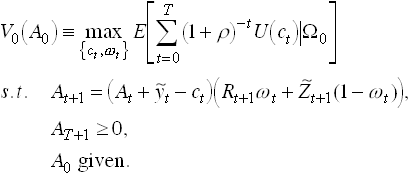
Use the Bellman equation

25
FOC:

Use the Envelope theorem

27
So
![]()
This is the Euler equation for consumption.

From we can also derive the result that all agents should invest in the risky asset if it has an expected return that is higher than Rt+1. This also if they have very high risk aversion. To see this write as

The Covariance term is zero when w is unity. So cannot hold then.
Some particular Euler Equations
Non-stochastic interest rate.

211
Quadratic utility

212

213
This is the Hall equation. No variable known in t is correlated with et+1. Can be tested using OLS.
The Hall Equation as a First Order Linear Approximation
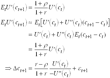
214
Note that low relative risk aversion and r>r gives high consumption growth. Why? Note also that by taking a first order approximation we disregard third moments in utility and second moments in consumption – certainty equivalence.
Examples of analytical solutions.
A. Quadratic utility, constant interest rate, only income risk, finite horizon.
Simplify r=r.
![]()
From intertemporal (collapsed) budget we know that

216
Then using we get

217
Certainty equivalence.
Look at r=r=0. Then perfect smoothing
![]()
218
This is the Modigliani Life Cycle Hypothesis.
Let T=¥ and r=r>0. Then

the Friedman Permanent Income Hypothesis.
No labor income, interest rate risk (multiplicative), CRRA (e.g. log), infinite horizon, time autonomous problem (z i.i.d.).
![]() .
This case we solved in MATFUII and showed that for log utility
.
This case we solved in MATFUII and showed that for log utility

220
where 1/(1+r ) is discount factor. Note that log Wt follows a random walk. A kind of certainty equivalence since for log utility income and substitution effects cancel.
C. Only labor income risk (additive) and normal i.i.d. innovations, finite horizon, CARA (exponential) utility. Simplify and set r=r=0. The consumer solves
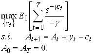
221
Assume a process for yt , for example
![]() .
.
with e t+1 N(0,s 2). Guess that
 .
.
By using that if ![]() then
then  we can check that this satisfies the
Euler equation. The budget constraint implies

With the expressions for expected consumption and income given by and , after taking expected values as of t, simplifies to

225
Note the problem with long and infinite horizons, consumption may be negative.
Quantifying Precautionary Savings
Take the Euler equation

Note that if U’ is convex the LHS is increasing in a mean preserving risk increase. Increases in risk thus has to be matched by decreasing consumption today and increasing expected consumption tomorrow. Both helps restore .
Do Taylor approximation of letting r=r

227
or

228
pa and pr are the absolute and relative coefficients of prudence.
Liquidity Constraints
All derivations above have assumed that the individual can save or borrow to smooth consumption so that the Euler equation is satisfied. But borrowing may, for several reasons, not be available in the required amount to make the Euler equation satisfied. In discrete time it is easy to show that the Euler equation for a period when the individual is liquidity constrained is given by
![]()
229
where we, just for simplicity assumed that the market interest rate coincides with the subjective discount rate. We let l t denote the shadow value (Lagrange multiplier) on the liquidity constraint that financial assets have to be non-negative (At ³ 0 " t). Certainly all extra income the individual receives in t will be consumed as long as l t > 0, i.e., as long as marginal utility today is higher than expected marginal utility tomorrow.
Now consider previous periods. Let us assume that the liquidity constraint is not binding then. For these periods the Lagrange multiplier is zero so the standard Euler equation holds implying
![]()
230
This means that the liquidity constraint affects consumption also in previous periods. Let us think of this as a three period problem. We then understand that some extra income in period t-1 will be smoothed out for consumption in period t-1 and t – over two, rather than three periods as in the non-constrained case. We thus see a higher propensity to consume out of income (but lower than 1) than in the risk-neutral non-constrained case. This is going to look exactly as if the individual reduced precautionary savings in response to a positive income shock. In empirical tests it is thus difficult or impossible to distinguish precautionary savings from potentially binding future liquidity constraints.
The Lucas Critique and Some Empirical Consumption Tests and Puzzles
The Lucas Critique
Sample moments between observed macro variables – like consumption, disposable income and output – change when policy change. This since optimum decision rules change with policy. Econometric models can thus only be used in short-term forecasting and can "provide no useful information as to the actual consequences of alternative economic policies".
MPC example
Assume that disposable income follows
![]()
231
Then

use then we may calculate MPC

If r is close to unity, MPC is close to unity. Now let there be a temporary lump sum transfer t to the house hold. A naive Keynesian would say that this increase consumption almost one for one. But,
![]()
Calculate MPC out of the transfer

235
So if MPC is estimated on income and then used to predict effects of fiscal policy we get wrong results (if r ¹ 0). Must have an economic model to understand the effects of policy changes.
A generalization of .
If
![]()
236
then
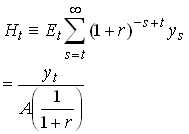
Tests and Puzzles
Hall -78
![]()
238
Can be tested by adding variables known in t to an OLS regression. Finds no influence from ct-1-s and yt- s. S&P stock market index has a significant influence. Suggested explanation – slow adjustments.
Carrol and Summers -89
Strong correlation long run growth in aggregate income and consumption in cross country study. Also at individual level. Appears that consumption grows one for one also with expected growth in income.
Potential explanations;
Liquidity constraints – must in such case be almost everybody. Most people have only very low financial savings.
Flavin -81, JPE
"Excess Sensitivity" to predicted changes in income.
Consumption change to predicted changes in income, e.g., when new pensions are paid out not when they are decided upon.
Campbell and Deaton -89
"Excess Smoothness".
Recall and . There we see that

239
C&D estimates a second order process for income

240
with r=0.442. An increase in growth signals future high growth. Then a shift in income today has a very large effect on permanent income so consumption should change very much. In this case
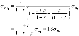
241
Instead they find that the coefficient is around 1 and only 1/2 for non-durables. So consumption is excessively smooth. This relies on non-stationary income.
Excess sensitivity and excess smoothness is two sides of the same coin. When expected future income increases consumption rise less then permanent income but responds when expectations are realized.
Caballero QJE -90 discusses precautionary savings as an explanation for excess sensitivity and excess smoothness. Assume that expected volatility of future earnings increase in the level (e.g., if y is a log random walk). Then a positive shock to expected future earnings increase precautionary savings so consumption does not respond one for one. When realized risk disappears so consumption increase.