Asset Pricing
In the previous sections we used the Euler equation to derive optimal consumption and investment decisions. Now note that the Euler equation defines a relation between consumption (or other real variables) and prices.
![]()
242
Previously we took the prices as given and derived the optimal path of consumption. We may, however, use the Euler relation in the other direction. Take the path of real variables, e.g., consumption as given and derive what the prices have to be. A straightforward way to do this is to assume that output is exogenous, like manna from heaven, and cannot be stored. In that environment we may introduce markets for capital and production facilities. This is the setup in the seminal Lucas (Econometrica, 1978) paper.
We will later relax the assumption about exogenous and non-storable output. This will give us the basic stochastic growth (or RBC) model.
Asset Pricing in the Lucas Tree Model and other CAPM
Asset Pricing in the Lucas Tree Model
Large number of identical agents.
Equal number of trees with stochastic crop dt The distribution of dt is Markov. Distribution is
. The process known by all agents.
Purpose: find pt – the price of a tree as a function of the state of the economy (dt).
The gross return on a tree is
(per capita)
No safe asset.
Perfect market in ownership of trees. All equal so no trade in equilibrium.
No storage or foreign trade so consumption ct = dt
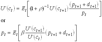
Substitute for ![]() from the Euler equation noting that w =0 gives
from the Euler equation noting that w =0 gives
243
By 7)

For any type of expectations in based on dt we
can compute a price today as a function of dt Let the
individuals subjective expectations of dt+1 be described
by ![]() and the
expectations about the relation between pt+1 and dt+1
be given by the function ps(dt+1). We then have
and the
expectations about the relation between pt+1 and dt+1
be given by the function ps(dt+1). We then have

Now Lucas defined the very powerful concept of rational
expectations. Let’s require that ![]() and
and ![]() . Lucas proves that this together with defines a unique
and constant pricing function
. Lucas proves that this together with defines a unique
and constant pricing function ![]() .
.
Use recursions on

A discounted sum of dividends. Stochastic discount rates unless marginal utility is constant.
A simple example with log utility

247
With dt i.i.d. so ![]()

248
Note that the price increases in dt (if U is concave).
Assume an autocorrelation in dt then  depends on dt Both
income and substitution effect, with log utility they cancel.
The Consumption and market CAPM
Previously we found that

The second equation in implies
![]() .
.
250
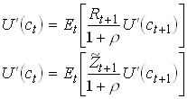
Substituting into the first equation in yields
251
Consider a similar problem but with n
risky assets each with a stochastic net return of ![]() (º
(º ![]() -1). FOC for each risk
asset i yields after the same substitution as above
-1). FOC for each risk
asset i yields after the same substitution as above

So

This is the Consumption CAPM.
So a risky asset can have an expected rate of
return that is larger or smaller than the safe return. Note that
a positive covariance between consumption and the risky return
implies a negative covariance between marginal utility and ![]() so that asset will
have a risk premium.
so that asset will
have a risk premium.
Note that if we have CRRA (![]() ) then we have
) then we have
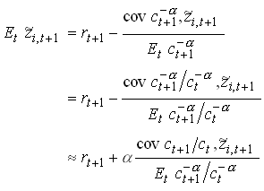
where I have used that ![]() .
.
Now assume there exists an asset m which return
is perfectly negatively correlated with marginal utility. So ![]() and thus
and thus ![]()
![]() .
.
Then from


Substitute into

This is the market or traditional CAPM.
Note that bi is the (true) regression coefficient in a
regression of asset i on m. The term ![]() can be interpreted as
the price of aggregate or systematic risk.
can be interpreted as
the price of aggregate or systematic risk.
Empirics
The Mehra – Prescott Puzzle
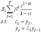
Consider a representative household that "maximizes"
258
l is
a stochastic growth rate that can take n different values ![]() all >0. The
probability of a specific growth rate depends only on last
periods growth rate.
all >0. The
probability of a specific growth rate depends only on last
periods growth rate.
![]() .
.
259
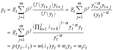
Assume there is a share that entitles the owner to the entire output the next period. From we have that the price of this share is
260
where i Î {1,...,n}. So the price is H(1) in c and y.
We can also use to get
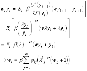
261
This is a linear equation system in n unknowns so we can solve it for the price of the share in all states of the world. Now we can calculate the net return on the asset

262
and expected return is

263
We can also compute the price of a safe asset in this economy.
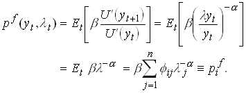
264
with a return of ![]() .
.
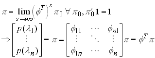
Now we want to find the unconditional (average) returns on the assets. First we need the unconditional probabilities of the states p.
Assume ergodic growth rates
265
Then

266
The risk premium is then defined as ![]() .
.
Results
Now simplify and assumed there is two states and a common transition probability.

267
Now we calibrate the model using the mean growth rate of GDP, its variance and autocorrelation.

268
Using these value and some reasonable values for b and a <10 we find that the risk premium should be something in the order of 0 to 0.4%. But on average the US stock market has yielded 6% more on average than government.
Consumption versus market b (Mankiw & Shapiro 1986)
Mankiw and Shapiro first estimates from 464
different stocks. They first estimate the market b, i.e., assuming it is
constant over time. Note that the coefficient on b should be
equal to the equity premium (around 6%) and constant for all
periods and assets. Then they use this variable to predict the
return on the corresponding asset.
![]()
269
The coefficient is significant and around 6 for most estimation methods.
Now rewrite

Assume that all relevant moments in are constant over time. We then bci as sample moments

271
Then we can run the regression
![]()
272
Now the estimate of g1 is insignificant and unstable. M&S also run a regression with both b, then only the coefficient on bmi comes out significant.