In general, preferences over consumption (bundles) at different points in time should be represented by a utility function of the form

1

The intertemporal elasticity of substitution between dates i and j is an evaluation of

2

This is straightforward to interpret. Compute the percentage change in the ratio of marginal utility at i and j that one percent change in the ratio of consumption at the same dates lead to. The inverse of the number is the intertemporal elasticity of substitution.

In general, however, is not sufficient to define the elasticity of substitution. The crux is that there is not a one-to-one mapping between the ratio of marginal utilities and the ratio of consumption. Then, since changing the ratio ci/cj can be done in many directions, i.e., an increase can achieved by increasing ci and/or decreasing cj. In the figure we want to see the effect of changing the ratio ci/cj starting from point x. An increase of the ratio to the one given by the ray 0-a’, can, fore example, be done by moving along any of the three arrows in the figure. These different directions will, in general have different effects on the ratio Uci/Ucj and thus produce different elasticities of substitution. One way out of this is to look at changes along the indifference curve, which would provide a compensated intertemporal elasticity of substitution. In the figure, this means moving along the arrow pointing northwest, which is tangent to the indifference curve at x. However, if we restrict attention to the class of homothetic functions, it is clear that the direction does not matter. Movement from point x, to any point on 0-a’ has the same effect on Uci/Ucj since the latter is constant along that ray. A widely used class of homothetic function is the CRRA class. On the other hand, the quadratic and the CARA class are not homothetic.

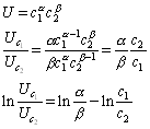
Now let us calculate the intertemporal elasticity of substitution for a homothetic utility function. Take an example

3

So

4

Now lets a make the assumption that

5

In the continuous time case, i.e., when the time period goes to zero this becomes

6

These are examples of additive time separability, i.e., that the function F(c1,c2,c3,…,cT) can be written .

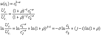
In and it is straightforward to define the rate of true time preference. This is rate at which future per-period-utility is discounted in the overall utility function. In the additively separable case, this is clearly distinct from the elasticity of substitution since it has nothing to do with how changes in consumption affect marginal utility. Take an example when the per-period-utility is CRRA.

7

or

8

so

9

which is independent of the rate of time preference.

Consider the class of additively time separable homothetic utility functions. Then, changing c1/c2 affects u’(c2) only if it affects c2. So, let us compute the elasticity of substitution by only changing c1. In this case

10

So

11

As you see, this is the inverse of the coefficient of relative risk aversion.

The assumption about time additivity is sometimes not appropriate. The simplest case would be to just let the period utility depend on current and the previous periods consumption, i.e.,

12

A bit more general example, that can capture habit formation is due to Campbell and Cochrane, is to include a time varying habit or subsistence level xt in the per period utility function

12

and let xt be a function of previous levels of consumption, for example

13

There is also ways of separating risk aversion within a period from intertemporal substitution. For example, in the two period case,

14

where it can be shown that the coefficient of relative risk aversion is h and the elasticity of intertemporal substitution is 1/e, which may be different from h.