MACRO I, 1998 SDPE

Lecture Notes

by John Hassler

CONTENT

• I. A Consumption, the Current Account and Risk

• I. B Fiscal Policy, Life Cycles and OLG Models

• I. C. Asset Pricing and International Risk Sharing

• II. C Endogeneous Growth

© John Hassler, can be copied freely for educational use.

Consumption, Fiscal Policy and Risk

I.A Consumption, the Current Account and Risk

The Intertemporal consumption choice

Three steps in the development of consumption modeling

Keynesian

1.1

worked well in cross-section studies with a>0, 0<b<1. Not consistent with time series evidence. Led to

Permanent income (Friedman, -57) – Life Cycle (Modigliani) hypothesis.

1.2

Distinguishes life time wealth and transitory income changes. Relation between income and consumption depends on relation between income changes and lifetime wealth. Compare

1.3

No account taken for second moments, effects of uncertainty.

Consumption and investment under uncertainty.

Precautionary savings. Leland (-68), Kimball (-90)

Irreversible investments. Option value of Waiting. Pindyck (-91), McDonald & Siegel (-86).

Permanent Income, Precautionary Savings and Liquidity Constraints

Consider the problem

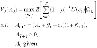1.4

Use the Bellman equation

1.5

FOC:

1.6

Use the Envelope theorem

1.7

So

1.8

This is the Euler equation for consumption.

Some particular Euler Equations

Non-stochastic interest rate.

1.9

Quadratic utility

1.10

1.11

This is the Hall equation. No variable known in t is correlated with e_t+1. Can be tested using OLS.

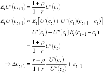1.12

Note that low relative risk aversion and r>r gives high consumption growth. Why? Note also that by taking a first order approximation we disregard third moments in utility an3d second moments in consumption – certainty equivalence.

A. Quadratic utility, constant interest rate, only income risk, finite horizon.

Simplify r=r.

1.13

From intertemporal (collapsed) budget we know that

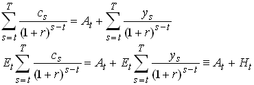1.14

Then using we get

1.15

Certainty equivalence.

Look at r=r=0. Then perfect smoothing

1.16

This is the Modigliani Life Cycle Hypothesis.

Let T=¥ and r=r>0. Then

1.17

the Friedman Permanent Income Hypothesis.

No labor income, interest rate risk (multiplicative), CRRA (e.g. log), infinite horizon, time autonomous problem (z i.i.d.).

For example, take the problem in , assume income is zero always, utility is log and time is infinite. Guess that the value function is given by

1.18

Substitute this into .

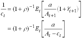1.19

which gives

1.20

Substituting this into the Bellman equation yields

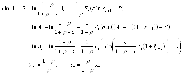1.21

where 1/(1+r ) is discount factor. Note that log W_t follows a random walk. A kind of certainty equivalence since for log utility income and substitution effects cancel.

C. Only labor income risk (additive) and normal i.i.d. innovations, finite horizon, CARA (exponential) utility. Simplify and set r=r=0. The consumer solves

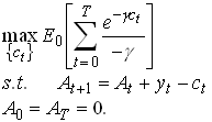1.22

Assume a process for yt , for example

. 1.23

with e t+1 N(0,s 2). Guess that

. 1.24

By using that if then we can check that this satisfies the Euler equation. The budget constraint implies

1.25

With the expressions for expected consumption and income given by and , after taking expected values as of t, simplifies to

1.26

Note the problem with long and infinite horizons, consumption may be negative.

Take the Euler equation

1.27

Note that if U’ is convex the LHS is increasing in a mean preserving risk increase. Increases in risk thus has to be matched by decreasing consumption today and increasing expected consumption tomorrow. Both helps restore .

Do Taylor approximation of letting r=r

1.28

or

1.29

pa and pr are the absolute and relative coefficients of prudence.

A Stochastic Model of a Small Open Economy

Some preliminaries:

Let us define the stock of net foregin assets at the end of period t as Bt+1. Equivalently, Bt+1 is the stock of foreign assets at the beginning of period t net of interest paid between period t and t+1. Then:

1.30

where Yt is aggregate income (except income on foreign assets), Ct is aggregate consumption and investments by domestic residents and the government and rtBt is the interest received on the stock of foreign assets that was held between period t-1 and t.

We now define the current account

1.31

which thus is the change in the holdings of foreign assets that took place during period t.

Let us define the permament value of a variable from the relation

1.32

so, for example, the permanent value of a variable income stream is the for ever fixed income level that would have the same expected PDV as the variable income stream.

Consider a representative individual that spends money on consumption C_t and investements I_t. There is also a government that consumes G_t. If this good enters the utility function of the individual, it enters additively, so the Euler equation is not changed.

Assume for now that the government applies taxes so its budget balances each period. The representative individual thus has a budget constraint given by

1.33

Collapsing this as in , taking expectations, assuming the no Ponzi condition and using the definition in

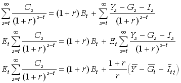1.34

The RHS can be thought of as the (net) wealth of the representative individual.

Now use the result from the previous section that in the risk-free case or under certainty equivalence (recall what could generate that) and when r=r>0, the Euler equation for consumption implies a consumption with a level that is expected to be constant. In this case this means that,

1.35

Now use this in the definition of the current account to get

The fundamental current account equation

1.36

So the current account is in surplus if Y_t is above its permanent level or if government consumption or investments is below their permanent levels. Can you provide the intuition for this?

Now let the effects of output shocks. Assume that income follows the stochastic process

1.37

We can then use result that

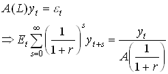1.38

So, for example, if the

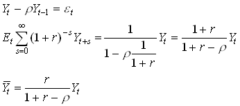1.39

The effect on the current account then becomes,

1.40

Similarly, when

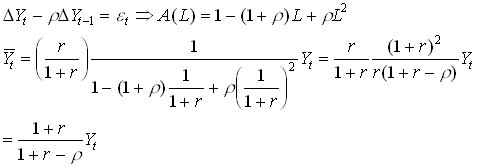1.41

So, if r larger than zero, permanent income fluctuates more than temporary. In this case,

1.42

so the effect on the current account by an unexpected increase in income is negative. The intuition is that if r larger than zero, an increase in income that is noted today, signals even larger income in the future. So, consumption increases to take also that increase into account.

We have so far treated investments as unaffected by the shock to Y. In reality, there may, of course, a correlation. For example, if a shock to Y_t increase the marginal productivity of capital, investments may increase in order to increase the capital stock. A way to model this is that

1.43

Now, if A_t increases permanently, this raises marginal productivity, which raises investments. Then, the current account must be negative in t. This since investments are above their permanent level and output is no higher than its permanent level.

The Lucas Critique Some Empirical Consumption Puzzles

The Lucas Critique

Sample moments between observed macro variables – like consumption, disposable income and output – change when policy change. This since optimum decision rules change with policy. Econometric models can thus only be used in short-term forecasting and can "provide no useful information as to the actual consequences of alternative economic policies".

MPC example

Assume that disposable income follows

1.44

Then

1.45

use then we may calculate MPC

1.46

If r is close to unity, MPC is close to unity. Now let there be a temporary lump sum transfer t to the house hold. A naive Keynesian would say that this increase consumption almost one for one. But,

1.47

Calculate MPC out of the transfer

1.48

So if MPC is estimated on income and then used to predict effects of fiscal policy we get wrong results (if r ¹ 0). Must have an economic model to understand the effects of policy changes.

Tests and Puzzles

1.49

Can be tested by adding variables known in t to an OLS regression. Finds no influence from ct-1-s and yt- s. S&P stock market index has a significant influence. Suggested explanation – slow adjustments.

Strong correlation long run growth in aggregate income and consumption in cross-country study. Also at individual level. Appears that consumption grows one for one also with expected growth in income.

Potential explanations;

Liquidity constraints – must in such case be almost everybody. Most people have only very low financial savings.

"Excess Sensitivity" to predicted changes in income.

Consumption change to predicted changes in income, e.g., when new pensions are paid out not when they are decided upon.

"Excess Smoothness".

C&D estimates a second order process for income

1.50

with r=0.442. An increase in growth signals future high growth. Then a shift in income today has a very large effect on permanent income so consumption should change very much. In this case

1.51

Instead they find that the coefficient is around 1 and only 1/2 for non-durables. So consumption is excessively smooth. This relies on non-stationary income.

Excess sensitivity and excess smoothness is two sides of the same coin. When expected future income increases consumption rise less then permanent income but responds when expectations are realized.

Caballero QJE -90 discusses precautionary savings as an explanation for excess sensitivity and excess smoothness. Assume that expected volatility of future earnings increase in the level (e.g., if y is a log random walk). Then a positive shock to expected future earnings increase precautionary savings so consumption does not respond one for one. When realized risk disappears so consumption increase.

1.B Fiscal Policy, Life Cycles and OLG Models

Ricardian Equivalence with zero birth rate or altruism

Above, in equation , we assumed that the government financed its spendings by taxing in an amount to generate zero deficits in each period. Now let us discuss whether relaxing this assumption can change our results. In particular, does the timing of taxes matter for consumption and the current account when we hold the stream of government consumption fixed? As before, we assume that the government goods do not interact with other goods in utility or production and disregard exogenous growth in population or technology. Let us do this in continuous time for a change.

The government budget constraint is

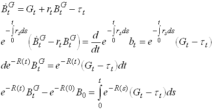1.52

where BG denotes the government deficit. Now require that the present value of the debt converges to zero (No Ponzi):

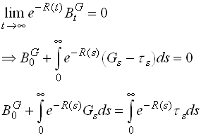1.53

So the present value of all future taxes equals the present value of future government spendings plus current debt stock.

Now look at the consumers. Recall that the slope of the consumption path was given from the Euler equation.

1.54

As long as the tax does not affect the return on savings, this condition is unaffected by the sequence of taxes.

Now look at the budget constraint. The continuous time version of with taxes instead of government consumption is

1.55

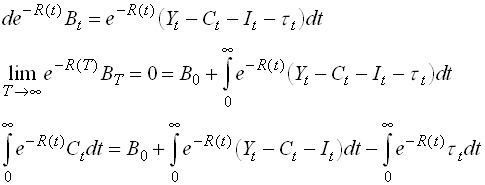
where B is the private sectors holdings of foreign asset. Integrate

1.56

Now we can substitute into the last line of

1.57

so we see that what is important for the households is only the present value of government spending plus initial foreign debt of the government. An implication of this is the following: assume the government change its fiscal policy so for given consumption is borrows more and taxes less. The private sector will then get a stock of assets in the form of government bonds. This stock is, however, of zero value in the aggregate. Thus the title of Barro's original paper. "Are government bonds net wealth?". Similarly, if the initial government debt was held by domestic agents, we would add B0G to the initial wealth of the consumer. This would cancel with the -B0G in .

What about the current account if the government decides to, say, increase taxes today by Dt? First consider the case when the government borrows or invests abroad. Then from we have that

1.58

Similarly, from

1.59

The current account in the continuous case is the sum of private and public rates of accumulation of foreign assets

1.60

and from and we see that the current account is unchanged. If the government borrows and lends to its domestic citizens, then the interpretation of changes so B is sum of foreign assets and government bonds (BG). The current account is still given by the accumulation of foreign assets, which now becomes the accumulation of total assets minus the accumulation of government bonds. Thus, the current account is still given by , which is unchanged by the change in taxes.

Some critical assumptions for the Ricardian Equivalence result

• Perfect capital markets (so the individual can save or borrow to offset any changes in the time path of taxes and deficits. Same interest for government and individuals.
• Taxes are lump sum.
• Infinite horizons and no new-coming generations, not necessarily infinite lives.

Ricardian Equivalence with Finite lives and altruism

Consider the simplest example of this. Each generation lives for one period, cares about their kids, who have the same per period utility function.

1.61

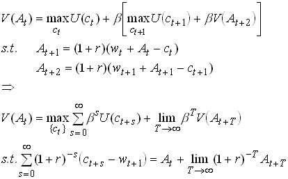
Now we can substitute from future generations problems

1.62

As you see, this is mathematically equivalent to dynamic optimization problem with infinite horizons. So the solution to this problem must be unaffected by the financing path of the governments consumption. Note that we require perfect capital markets. In this context it in particular requires that At may be negative or that households choose positive values (bequests) voluntarily.

Fiscal Policy in a Small Open Economy OLG Model

Consider a very simple version of the Samuelson-Diamond-Blanchard OLG model.

Households

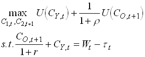
Live for two periods and solve

1.63

where tt is taxes levied on the young in period t. The household consumption function is increasing in both income and the interest rate since each young generation consist of net savers.

1.64

The economy is small and open so factor prices are exogenous. Assume for simplicity that the economy's net assets are invested abroad. Without a government, we then have

. 1.65

So, the current account is

1.66

Now assume there is a government that taxes and transfers money. If there is a deficit it borrows from the current young generation. Now consider the following fiscal policy experiment.

First, the government unexpectedly transfers T in period t to the old and finance it with a deficit, i.e., it borrows from the currently young. It then rolls over the debt but issues taxes on the young to raise money for the interest. The consumption of the old generation in period t increases by T. What about the young in t?. By assumption, tt=0, so their budget constraint is unchanged so their consumption must be unchanged.

What happens to the current account? The savings of the young is now taking two forms, one part is in foreign assets and one in bonds. (Why are the bonds net wealth here?) So,

1.67

Alternatively, if the government borrowed abroad, would still be true if we let Bt+1 include the government holdings of foreign assets. And

1.68

Note that this is equal to private savings plus public savings

1.69

since the savings of the young is unchanged, the savings of the old is unchanged (their income including transfers increases with the same amount as the consumption),. while the government have a deficit (negative saving) of T. Thus, the expansionary fiscal policy, leads to a current account deficit.

What happens after t+1? Each new young generation lends T to the government, gets it back when they are old and are taxed to pay the interest rate. Thus, ts=rT, for all s>0. So their consumption must be

1.70

Clearly, consumption smoothing implies that the consumption falls relative to CY,t by an amount inside the interval (0, Tr). The lower limit is consumption is not affected, i.e., all consumption reduction by the generation born in t+1 is done when they are old. The upper limit if is all consumption reduction is done when they are young. Consumption smoothing implies that the true effect is in-between these two limits. So:

1.71

Note, that the negative effect on the current account in t+1 can be understood as the government taxing people with a low propensity to consume (young) and gives the receipts to people with high propensity to consume (old). Again, an expansionary fiscal policy reduces the current account.

What happens after t+2? Each new young generation lends T to the government, gets it back when they are old and are taxed to pay the interest rate to the currently old. So they face the same budget constraint and the current account is zero. So clearly, the policy experiment has reduced the stock of foreign assets.

The intuition for the breakdown of Ricardian Equivalence is that a budget deficit is a way to transfer resources between generations. In general, a government spending plan should be financed by a mortgage with the same pay-back period as the life span of what is financed not to cause intergenerational transfers. E.g., a bridge that lasts 50 years should be financed with a 50 year mortgage.

Note that we can interpret the experiment as a Pay-as-you-go pension system.

A Large Economy OLG model

Let us now consider a closed economy, where factor prices are determined as equilibrium outcomes at domestic factor markets.

Households

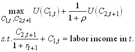
Live for two periods and solve

1.72

Firms

Hire labor and capital on competitive market and combine them in a CRS production function to produce the only good. This is sold on a competitive market to the households.

Firms solve

1.73

where At is a productivity index that grows geometrically at rate g. We can think of AL as the number of effective units of labor. Also L grows at a geometric rate n. So

1.74

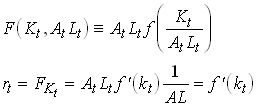
The competitive market imply that factors are paid their marginal products. r = FK and w=FAL.

Since F is H(1) we have

1.75

So f is production per effective labor unit and k is capital per effective labor unit. Note that

1.76

Since we CRS and competitive markets firms make zero profits. We can write this as

1.77

Note that we now see that both wages and interest rates are determined by the current capital to effective labor ratio. We thus write

1.78

Capital market

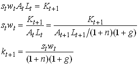
The labor income of a young generation in t equals wt At Lt . Part of this is consumed (c1,t) and the rest is saved. Let st denote the share of labor income that is saved. This will, in general depend on labor income and the interest rate. The savings in period t is next periods capital stock

1.79

Now assume that st only depends on rt+1. (Which class of utility functions produce this result? What are the effects of higher r?) Then we can write the last line of as

1.80

This (implicitly) defines a difference equation for k, i.e., a relation between kt and kt+1 that has to be satisfied in this model. Note that if we made the Solow assumption of a constant savings rate, the difference equation takes an explicit form. Since in this case the RHS contains no kt+1. Fortunately there is a utility function for which the income and substitution effects of higher interest rates cancel so that the household will choose a constant savings rate regardless of the interest rate.

Functional specification

Let us look at a particularly simple specification. Assume U is the log function and that that production is (Wicksell-) Cobb-Douglas, .

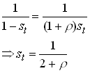
Now we can write the consumption decision of the consumer as follows.

1.81

with foc

1.82

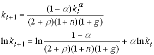
Now we only need to specify the wage function to have an explicit version of . We see immediately that. So becomes

1.83

Can you solve this difference equation and is it stable? Here is an example of a plot of .

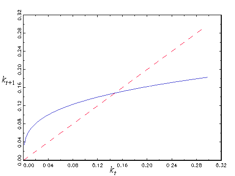
The steady state of is its fixed point

1.84

The interest rate in steady state is

1.85

Dynamic Inefficiency

In each time period the amount of resources is Kt + F(Kt ,AtLt). This has to be split into aggregate consumption and next periods capital stock. We can than write

1.86

where Ct is total consumption of young and old in period t. Now divide by At Lt

1.87

ct is aggregate consumption per unit of current effective unit of labor.

Now consider an economy in a steady state. We then have

1.88

Let us find the value of the steady state capital stock that maximizes aggregate consumption per effective unit of labor. The FOC for this problem is

1.89

This is a variant of the Ramsey Golden Rule. A steady state capital stock above kgr is not Pareto efficient. If we are above kgr we could increase aggregate consumption in all periods now and in the future by reducing forcing the steady state capital stock to be lower.

Now compare and

1.90

So it is possible that the economy is not on the Pareto frontier and thus dynamically inefficient. What goes wrong here and why does not the first welfare theorem hold? One way of understanding this is to realize that the only way a young generation can reduce the capital stock is by saving less but then consumption would have to be lower for them in the second period. If, however, there was a mechanism that specified that young people saved less but in return got some transfers from the young next period, everybody could be made better off. What does this remind you off?

Borrowing versus Taxing in the standard OLG model

Now let us look at whether Ricardian Equivalence holds in a standard OLG model without altruism. To focus on the path of financing rather than the spending side we consider a government which wants to finance a constant spending level of 0 for convenience. Consider a government that issues debt equal to Tt , gives the proceeds to the currently young, rolls over the debt for ever and the tax the young in all future periods to pay the interest rate minus the growth rate of the economy. This means that tt will be held constant at a level t. For simplicity let us use the log utility, Cobb-Douglas production specification.

The saving decision of the currently young given in is unaffected but the transfer has to be added to the wage

1.91

From this we see that current consumption increases when the policy is started up. Total savings also increase and become

1.92

Note that part of the savings is in form of government bonds. But it is only real savings that translate into next periods capital stock. To put it differently next periods capital stock is equal to private savings plus government savings, the latter being equal to minus Tt

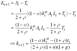1.93

Alternatively we could derive from noting that next periods capital stock equals production plus the capital stock minus consumption.

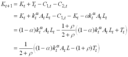. 1.94

From we see that it is clear that the deficit financed transfer causes next periods capital stock to decrease. This means that the interest rate goes up. This in turn means that the old in the next period can consume more for each dollar saved when young. Since total savings (the sum of real and financial savings) increased, the old in t+1 will consume more. The generation born in time t when the debt was issued will this clearly benefit and we do not have Ricardian Equivalence.

From next period the government takes away an amount equal to the debt plus interest rate from the young and gives them the rolled over debt. Let Ht+1 denote total wealth of a generation born at t+1. We then have

1.95

We see that wealth decrease (increase) in t if the economy is dynamically efficient (inefficient). This is for given kt+1 Since the introduction of a government debt necessarily implies a lower capital stock this has negative effects on the wealth and utility of the young in t+1. For sufficiently large dynamic inefficiencies it is possible that that the first effect dominates for small debt levels.

Now consider the consumption of the young;

1.96

and consumption of the old is

1.97

Now consider the capital accumulation equation. This equals total resources available minus consumption

1.98

Normalizing and simplifying we get

1.99

This follows from the fact that next periods capital stock is equal to the share of production that goes to the young minus their consumption. We see that this difference equation implies that next periods k is lower the larger is t. This implies that the new steady state capital stock is necessarily smaller when a debt roll-over is introduced.

I.C. Asset Pricing and International Risk Sharing

In the previous sections we used the Euler equation to derive optimal consumption and investment decisions. Now note that the Euler equation defines a relation between consumption (or other real variables) and prices.

1.100

Previously we took the prices as given and derived the optimal path of consumption. We may, however, use the Euler relation in the other direction. Take the path of real variables, e.g., consumption as given and derive what the prices have to be. A straightforward way to do this is to assume that output is exogenous, like manna from heaven, and cannot be stored. In that environment we may introduce markets for capital and production facilities. This is the setup in the seminal Lucas (Econometrica, 1978) paper.

We will later relax the assumption about exogenous and non-storable output. This will give us the basic stochastic growth (or RBC) model.

CAPM and the Lucas Tree Model and other

• Large number of identical agents.
• Equal number of trees with stochastic crop dt The distribution of dt is Markov. Distribution is. The process known by all agents.
• Purpose: find pt – the price of a tree as a function of the state of the economy (dt).
•  
• The gross return on a tree is (per capita)
•  
• No safe asset.
•  
• Perfect market in ownership of trees. All equal so no trade in equilibrium.
• No storage or foreign trade so consumption ct = dt

Substitute for from the Euler equation gives

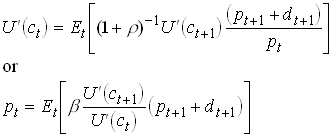1.101

By 7)

1.102

For any type of expectations in based on dt we can compute a price today as a function of dt Let the individuals subjective expectations of dt+1 be described by and the expectations about the relation between pt+1 and dt+1 be given by the function ps(dt+1). We then have

1.103

Now Lucas defined the very powerful concept of rational expectations. Let’s require that and . Lucas proves that this together with defines a unique and constant pricing function .

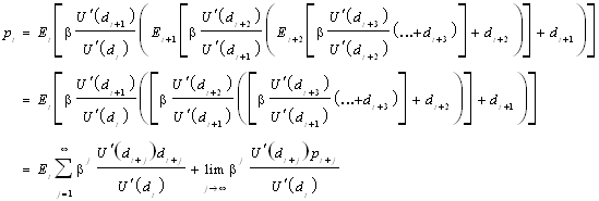
Use recursions on

1.104

A discounted sum of dividends. Stochastic discount rates unless marginal utility is constant.

A simple example with log utility

1.105

With dt i.i.d. so

1.106

Note that the price increases in dt (if U is concave).

Assume an autocorrelation in dt then depends on dt Both income and substitution effect, with log utility they cancel.

Consider a slight addition to the problem , namely that individuals can invest a freely chosen share w of their assets in a risky asset and the remainder in the risk free asset. We assume away other income. The asset accumulation becomes

1.107

and the Bellman equation

1.108

Using the envelope theorem to substitute for V’, the first order conditions are

1.109

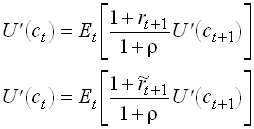
The second equation in implies

. 1.110

Substituting into the first equation in yields

1.111

Consider a similar problem but with n risky assets. FOC for the portfolio share in each risk asset i yields

1.112

So

1.113

This is the Consumption CAPM, yielding the equilibrium expected return that must result on a competitive market.

So a risky asset can have an expected rate of return that is larger or smaller than the safe return. Note that a positive covariance between consumption and the risky return implies a negative covariance between marginal utility and so that asset will have a risk premium.

Note that

1.114

where d is dividends and p is the price of the assets. So CAPM yields a relation between today’s asset price and the expected price tomorrow. CAPM is thus in itself not enough to pin down the asset prices. A no-bubble condition is also needed.

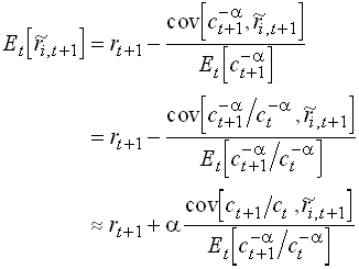
If we have CRRA () then we have

1.115

where I have used that .

Now assume there exists an asset m which return is perfectly negatively correlated with marginal utility. So and thus .

Then from

1.116

1.117

Substitute into

1.118

This is the market or traditional CAPM. Note that bi is the (true) regression coefficient in a regression of asset i on m. The term can be interpreted as the price of aggregate or systematic risk.

Empirics

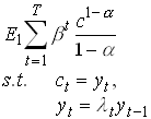
Consider a representative household that "maximizes"

1.119

l is a stochastic growth rate that can take n different values all >0. The probability of a specific growth rate depends only on last periods growth rate.

. 1.120

Assume there is a share that entitles the owner to the entire output the next period. From we have that the price of this share is

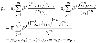1.121

where i Î {1,...,n}. So the price is H(1) in c and y.

We can also use to get

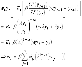1.122

This is a linear equation system in n unknowns so we can solve it for the price of the share in all states of the world. Now we can calculate the net return on the asset

1.123

and expected return is

1.124

We can also compute the price of a safe asset in this economy.

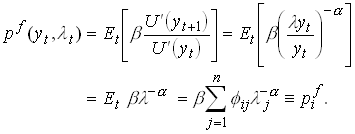1.125

with a return of .

Now we want to find the unconditional (average) returns on the assets. First we need the unconditional probabilities of the states p.

Assume ergodic growth rates

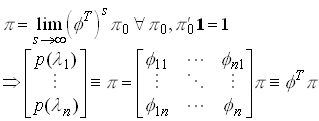1.126

Then

1.127

The risk premium is then defined as .

Now simplify and assumed there is two states and a common transition probability.

1.128

Now we calibrate the model using the mean growth rate of GDP, its variance and autocorrelation.

1.129

Using these value and some reasonable values for b and a <10 we find that the risk premium should be something in the order of 0 to 0.4%. But on average the US stock market has yielded 6% more on average than government.

Mankiw and Shapiro first estimates from 464 different stocks. They first estimate the market b, i.e., assuming it is constant over time. Note that the coefficient on b should be equal to the equity premium (around 6%) and constant for all periods and assets. Then they use this variable to predict the return on the corresponding asset.

1.130

The coefficient is significant and around 6 for most estimation methods.

Now rewrite

1.131

Assume that all relevant moments in are constant over time. We then bci as sample moments

1.132

Then we can run the regression

1.133

Now the estimate of g1 is insignificant and unstable. M&S also run a regression with both b,  then only the coefficient on bmi comes out significant.

International Risk Sharing

Consider a world with N countries indexed by n, inhabited with individuals with identical CRRA utility functions. Each country has a production sector that yields a stochastic output in each period, denoted Ytn. Shares in the production sector are traded on the world market where there is also a risk free on period bond traded with a safe return rt+1 between period t and t+1. . Buying a share in country n’s production sector in period t, yields a stochastic return. The problem is

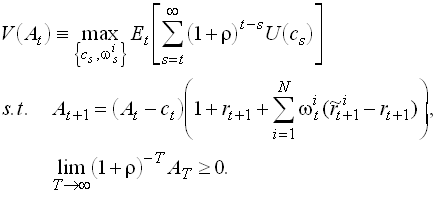1.134

The Bellman Equation becomes

1.135

The first order condition for optimal portfolio shares is

1.136

Now assume log utility and use the result in to guess that the value function is aln(A) + b. (Make sure you know how to verify the guess). Then we get

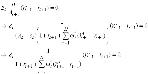1.137

This is a complicated equation to solve, but we can see one thing immediately. The equation does not involve individual wealth. This means that all individuals, regardless of where they live, should choose the same portfolio shares. In other words, the individuals in each country should simply hold a portion of the world portfolio of assets. This results remains if we use CRRA functions with elasticities different from unity.

The equal portfolio shares result is grossly at odds with the empirics. For example, the average US investor held 94% of her wealth in domestic assets. The predicted share is much lower. This is called the home-bias puzzle. The gain from diversifying may be large – in 1987 an average return of 10% with a standard deviation of 17.3% on the S&P500 could be transformed into an average return of 13% with a standard deviation of less than 16% by using 14 non-US bond and equity markets.

Attempted explanations for the home-bias puzzle

1. Non-traded goods.
2. Restrictions and frictions.
3. Irrational behavior.
4. Informational asymmetries.

II. Economic Growth

II.C Endogenous Growth

Prerequisites for Endogenous Growth

Take the simplest neo-classical growth model and assume away the exogenous growth rates in A and L. Can we anyway generate sustained long run growth? Let the CRS production function be

2.1

and capital accumulation

2.3

Now

2.4

Now , what happens to gy as time goes to infinity. The RHS of is non-negative. As long as s is strictly positive, capital accumulation continues. So if s is kept positive FK falls forever since FKK <0. In other words, if F shows CRS in K and AL, then it shows DRS in K alone. If the Inada condition

2.5

then the economy thus is bound to approach zero growth due to and the fact that s is finite.

With depreciation or population growth we need that the limit in is large enough to account for depreciation and population growth.

What is the fix? We need to have a production function that shows CRS in factors of production that are produced (i.e., that are accumable). The most simple and straightforward way is to let the productivity index A depend on how much capital the economy has accumulated. We could think of this as a Learning by doing mechanism.

So in the simplest endogenous growth model we could assume that the level of knowledge, measured by A is given by

2.6

Substituting into the production function we have

2.7

From the CRS assumption we have

2.8

The term F(1,aL) is constant so output is linear in K alone, i.e., shows CRS in K alone. In some of the already classic articles by Romer and others the constant was called A. Then we can write Y=AK, thus these models go under the name AK-models.

The basic ingredient in endogenous growth models is thus to construct a social production function that has CRS in produced factors of production. There are basically to lines of models that achieve this,

1. Knowledge or Human Capital in the production function. Knowledge and/or human capital is surely producable as you hopefully experience during this course. If then the production function has CRS in capital and human capital together.
2. Increasing specialization. Since Adam Smith we know that increasing market sizes permits increasing specialization. So as production increases the economy may be more and more efficient. This may be another source of endogenous growth.

Growth rate in the simplest learning by doing (AK) model

Let the constant F(1,aL) be called A. Then we have

2.9

So the growth rate of the economy depends on the growth rate of capital which in turn depends on the net savings rate. With a given savings rate s

2.10

In this simple model it is easy to endogenize the savings decision. With CRRA preferences

2.11

the Euler equation, which we can derive using Optimal Control, states that

2.12

where rt is the net return on savings. If this equals the full marginal return on capital (why should it not?) – rt = A so

2.13

The only saving rate which is consistent with and the transversality conditions is that the growth rate of consumption equals the growth rate of output. What would happen otherwise? So

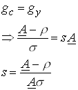2.14

Note that this model implies very simple dynamics – the economy is always in its steady state growth path. Shifts in some parameters or a shock to the capital stock implies an immediate jump to the new steady state growth path. Can you explain why?

Variations

Aggregate versus Private Knowledge

In the previous example there was no distinction between aggregate and private knowledge. This meant that the learning by doing effect of accumulating capital was fully internalized in the savings decision by the individuals. This may, reasonably, not be the case. Take the opposite view instead. Assume that there are an infinite number of identical small firms indexed by the rational numbers i on a unit interval [0,1]. Now that the production function for the individual firm is given by

2.15

The level of knowledge is proportional to the aggregate stock of capital and is identical to all firms.

2.16

Now the aggregate production function can be written

2.17

However, when a firm decides to increase its capital slightly, the effect that has on the aggregate capital stock and thus on the stock of knowledge is negligible. This since

2.18

So the private return on capital is

2.19

which is smaller than the social which equals

2.20

Let, for example, the production function be

2.21

The private return to capital is in this case

2.22

Since this is the interest rate faced by consumers the Euler equation for consumers with CRRA utility gives

2.23

So we see that growth in this model is to low compared to the welfare maximum given by

R&D

In the previous examples knowledge was produced as a by-product of capital accumulation. We can easily change that and introduce a specific sector where knowledge is produced. So let

2.24

where aL is the share of labor that is allocated to knowledge accumulation. This sector could be thought of as an R&D sector or a schooling sector. The are some decreasing returns to scale in this sector if g is smaller than unity. The production function for output and the capital accumulation is given by

2.25

For now we assume that savings and the share of labor allocated to R&D is fixed and exogenous. Now lets define

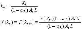2.26

So, as in the Solow model

2.27

Now this reminds us about the Solow model and a steady state occurs when is zero. Let us look at a plot of the components in the RHS of .

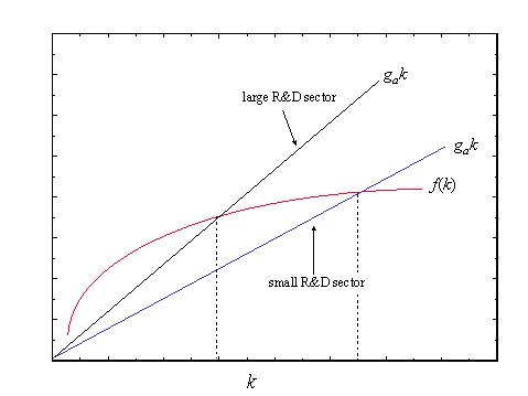
We see that a large R&D sector and thus a high growth rate of knowledge implies a lower steady state capital/effective labor ratio and vice versa. What would happen if we got a shift from a low to a higher share of labor in the R&D sector?

In this model the savings rate is unimportant for long run growth as in the Solow model. But, now growth is (almost) endogenous. To really explain growth we would like to let aL be determined within the model. This is the next step in the development of this model. We would like to have some firms who do the R&D and hire labor for this. Obviously we need to introduce some property rights for that purpose. Note that in such a model there is no reason to believe that growth is at its socially optimal level.

Growth from increasing specialization

Now let us turn to the other source of sustained growth – specialization. Let us think of an economy with two sectors. Final output which is produced using labor (with inelastic supply) and a range of intermediate goods. The latter are produced with capital only. The production function for the final good is

2.28

where each xi,t represents the amount of a particular intermediate input that is used at time t. Mt is the total number of intermediate inputs in use at t. We are going to look at symmetric equilibria where all xi,t are equal and denoted xt so

2.29

where we have normalized the labor supply to unity. The specification in implies that there is positive returns to specialization. Consider the case when we double the number of inputs but use each in half the amount. Output is then

2.30

Now look at the intermediate goods production sector. Here capital is transformed into intermediate goods by Mt firms. There is a fixed cost of running a firm (paid in capital) so the capital requirement of firm i which produces xi,t can be written

2.31

Now we assume that the final goods sector is competitive and that it buys intermediate goods so that its marginal product equals its price

2.32

This is the inverse demand faced by the intermediate goods producing firms so their profits are

2.33

where rt is the user cost of capital (interest rate plus depreciation). From follows that the profit maximum for intermediate goods producing firms is

2.34

where the last equality comes from the assumption of a symmetric equilibrium. Now assume that there is no barriers to entry so profits in the intermediate goods sector are zero.

2.35

Lastly, we require that the capital market is in equilibrium so that supply of capital (which is given at any point in time) equals its demand. This implies

2.36

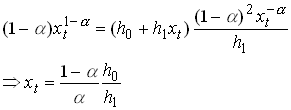
Substituting from into we get

2.37

Lastly, substituting this into we get

2.38

Substituting these results into the production function for aggregate output we get

2.39

so we are back into the simple AK model. Now we just have to make some additional assumption about savings, for example that it is chosen optimally by individuals facing some interest rate, for example the one established at the capital market and given by if there are no capital income taxes. That savings rate determines the growth rate of capital which from is identical to the growth rate of output.